Icon Set Alternative

I'll be honest. I never use icon sets. But I had a look at them the other day and thought that they didn't do what I expected.

Here's a screenshot of them in action.



For those not familiar, icon sets are used the following way. Select the range of cells you want to add them to, then on the Home tab, select Conditional Formatting, Icon Sets and choose which one is best for you.



Let's see what they are actually doing. Select Conditional Formatting from the Home tab, then Manage Rules, select the rule in use (you should be able to see Icon Set on the right), then click Edit Rule.



Okay, it appears that the icons change according to what range of values they are in. I would prefer to see when values change regardless of range, so an ↑ arrow for increases, ↓ arrow for decreases and a → arrow if values stay the same.

It's easy enough to set up an alternative. First the arrows - I could use Wingdings 3 font to get some arrows, but I've decided to go a different way for formatting preference, and because it's easier to use actual arrow characters inside formulas, rather than use "g", "h" and "i", then try to remember what they refer to later on.

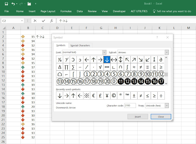
So I selected Symbol on the Insert tab, then selected the Arrows subset on the Symbol dialog box and inserted them into a cell for later use.



Jumping ahead, the next screenshot shows what I'm up to. I've entered the following formula from the second cell down in an adjacent column. Left or right, it's up to you. Note that I'm not including the top cell. Formulas and formatting start in Cell B3.



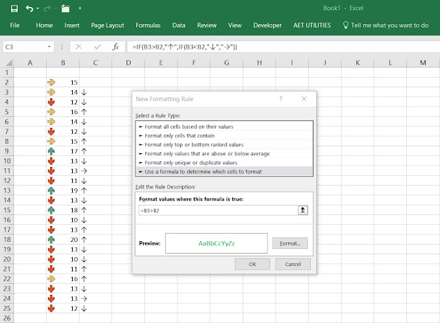
And as you can also see, I've entered a conditional format. Green if Cell B3 is greater than Cell B2. Note that for Conditional Formatting, you only need to use a TRUE condition. And as the whole range is selected, Conditional Formatting will adjust the condition's cell references to work with each cell accordingly.

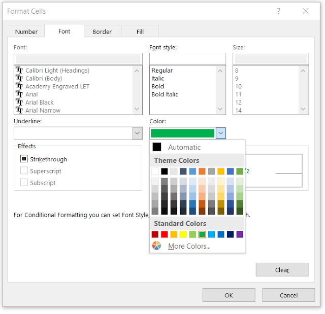
By the way, I formatted the font by clicking the Format button, then Color (Americans don't know how to spell. They did invent Excel though!) and selecting green from the pallette.



I do the same for when Cell B3 is less than B2, with the font becoming red.



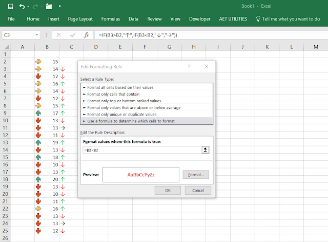
Almost there. I don't need 3 conditional formats, I just change the existing font colour in the cells themselves. Not Yellow, it's too hard to see. Orange is a better choice, and I also make the font bold to make the arrows stand out a bit more.



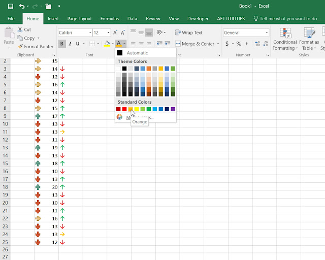
Done! See you next time.