Monthly Report Tutorial

At a former client, I was asked to submit monthly reports that show details of work performed in 15 minute increments.

My line of thought went something like this,

"Let's see, a monthly calendar, something like the one on my fridge door comes to mind and making one in Excel should be easy..."



One problem is space. If I do several tasks in one day, do I use tiny font to make the details fit, or do I make the calendar larger to the point that I have to scroll copiously?

Also, just how practical is that style of calendar going to be when it comes to adding up total time per task? Something along the lines of a regular timesheet would be better.

I can easily fit 32 rows on my laptop screen. That's a good start. So here's how to do the same thing I did, if you are interested.

Leave the first row for your headers. In cells A1 and B1, enter "Date" and "Day", then change the orientation. Right click the cells, select Format Cells, Alignment, and change Orientation to 90 degrees.



(You might want to change the Alignment too. Choose from the options on the Alignment Group on the Home Tab)

Enter the first day of the month in cell A2. Select range A2:A32, then change the format to either "d/m" or "m/d" as you prefer. Right click the cells, select Format Cells, Number, and enter the format in the Type text box in the Custom section.



Now enter =A2+1 into Range A3:A32 and click your Ctrl and Enter keys simultaneously to enter the formula into all selected cells.

In the same way, enter =CHOOSE(WEEKDAY(A2,1),"Su","Mo","Tu","We","Th","Fr","Sa") into Range B2:B32.

Adjust the width of both of these columns and set the alignment to suit.

You should have something like this.



And now for the details. Long descriptions take up space, so let's use numbers instead. Keep in mind that longer tasks won't be completed in 15 minutes, and recurring tasks will be duplicated so that's going to cut down the number of tasks in total. With any luck, we can keep things within double digits.

Start times allotted for the 15 minute intervals go in Row 1. Adjust the Orientation to 90 degrees. "h:mm" is a suitable format.



The task descriptions that match the numbers can go on the right. But note the numbers to their left to perform a lookup.



Important: adjust the following ranges to suit your requirements. Use Named Ranges if you prefer.

Enter formulas to add up the time. Type the following formula into Cell AI2, and drag down to the end of your list.

=IF(COUNTIF($C$2:$AE$32,AG2)=0,"",COUNTIF($C$2:$AE$32,AG2)/4)
You should have something like this.



You can freeze the first row if the number of tasks exceed the number of visible rows on your screen. (View Tab, Windows Group, Freeze Panes, Freeze Top Row)

Now for some extra features to enhance visibility. Why not add some Conditional Formatting to highlight the weekends? With Range A2:AE32 selected, click the Home Tab, Styles, Conditional Formatting, New Rule, then "Use a formula to determine which cells to format" and enter this formula. (Click the Format button to choose a suitable format)



Here's the result.



An ActiveX Combo Box and a bit more Conditional Formatting makes it easy to see when the work was done. If you can't see the Developer Tab on the Ribbon, select the File Tab, Options, Customize Ribbon, then tick "Developer" on the list to the right and click the OK button.



On the Developer Tab, select Insert from the Control Group to add an Active X Combo Box. (I've already added one to Cell AH1)



Right click the Combo Box and select Properties. Set the LinkedCell and ListFillRange properties. I've hard-coded my ListFillRange range reference but you can use Named Ranges too, as in "=Tasks" without the quotation marks.



When finished, toggle off Design Mode on the Developer Tab.

Note the linked cell. That gives me the selected item of the list. Now I use another formula to get the reference number which I have put in the cell below the linked cell (In this case, Cell AJ3).

=MATCH(AJ2,AH:AH,0)-1
If I select the first item on the Combo Box, Cell AJ3 will show 1.



Here's the Conditional Formatting for the details part of the report. (Range C2:AI32)



And here's the Conditional Formatting for the list. (Range AG2:AH32)



I also added some Data Bars to the hours.



And we're done.



No VBA was used so you can send the file without explaining the need to enable macros.

Here's a download link if you want to skip making one yourself.

Icon Set Alternative

I'll be honest. I never use icon sets. But I had a look at them the other day and thought that they didn't do what I expected.

Here's a screenshot of them in action.



For those not familiar, icon sets are used the following way. Select the range of cells you want to add them to, then on the Home tab, select Conditional Formatting, Icon Sets and choose which one is best for you.



Let's see what they are actually doing. Select Conditional Formatting from the Home tab, then Manage Rules, select the rule in use (you should be able to see Icon Set on the right), then click Edit Rule.



Okay, it appears that the icons change according to what range of values they are in. I would prefer to see when values change regardless of range, so an ↑ arrow for increases, ↓ arrow for decreases and a → arrow if values stay the same.

It's easy enough to set up an alternative. First the arrows - I could use Wingdings 3 font to get some arrows, but I've decided to go a different way for formatting preference, and because it's easier to use actual arrow characters inside formulas, rather than use "g", "h" and "i", then try to remember what they refer to later on.

So I selected Symbol on the Insert tab, then selected the Arrows subset on the Symbol dialog box and inserted them into a cell for later use.



Jumping ahead, the next screenshot shows what I'm up to. I've entered the following formula from the second cell down in an adjacent column. Left or right, it's up to you. Note that I'm not including the top cell. Formulas and formatting start in Cell B3.



And as you can also see, I've entered a conditional format. Green if Cell B3 is greater than Cell B2. Note that for Conditional Formatting, you only need to use a TRUE condition. And as the whole range is selected, Conditional Formatting will adjust the condition's cell references to work with each cell accordingly.

By the way, I formatted the font by clicking the Format button, then Color (Americans don't know how to spell. They did invent Excel though!) and selecting green from the pallette.



I do the same for when Cell B3 is less than B2, with the font becoming red.



Almost there. I don't need 3 conditional formats, I just change the existing font colour in the cells themselves. Not Yellow, it's too hard to see. Orange is a better choice, and I also make the font bold to make the arrows stand out a bit more.



Done! See you next time.

Text Troubles

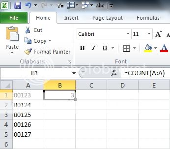
If you work with data from various sources, it's possible you will come across numbers formatted as Text. Depending on what you plan to do with these numbers, it's possible that the Text formatting will cause problems. For example, let's see how many "numbers" there are in the picture below. Look at the formula I've entered in cell B1.



Hmmm. Unlikely? No, I've been handed data apparently "managed" by 2 or more people, with different formatting within the same column. It does happen.

Let's set things right.

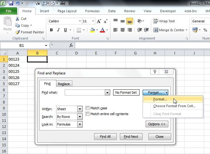
Clicking Ctrl + F on your keyboard brings up the Find and Replace dialog box. From there, click Format, then Format again.



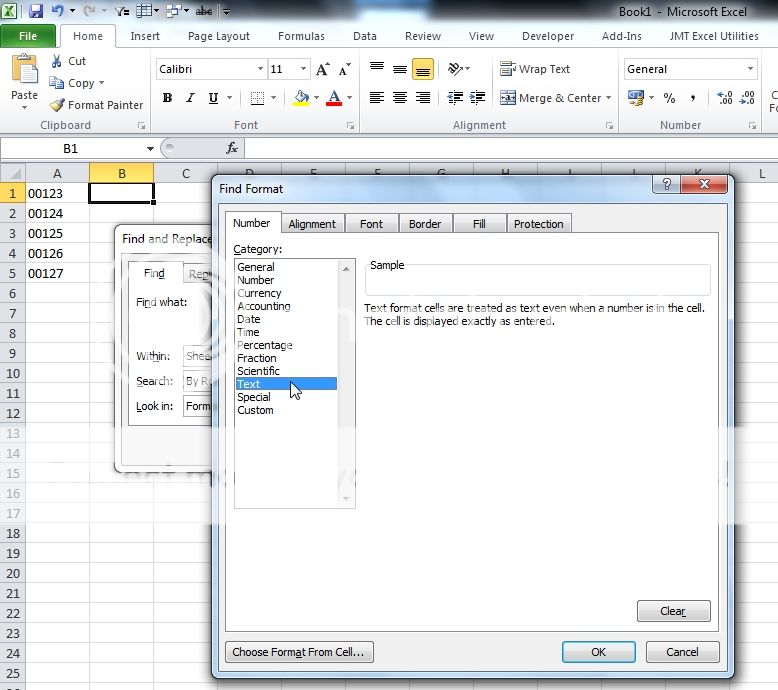
Select Text from the Number tab, then click OK.



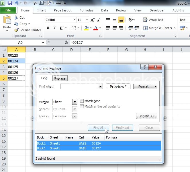
Click Find All, then type Ctrl + A on your keyboard to select all cells found with Text format.



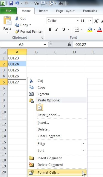
Bring up the right-click menu with your mouse (or keyboard) and select Format Cells.



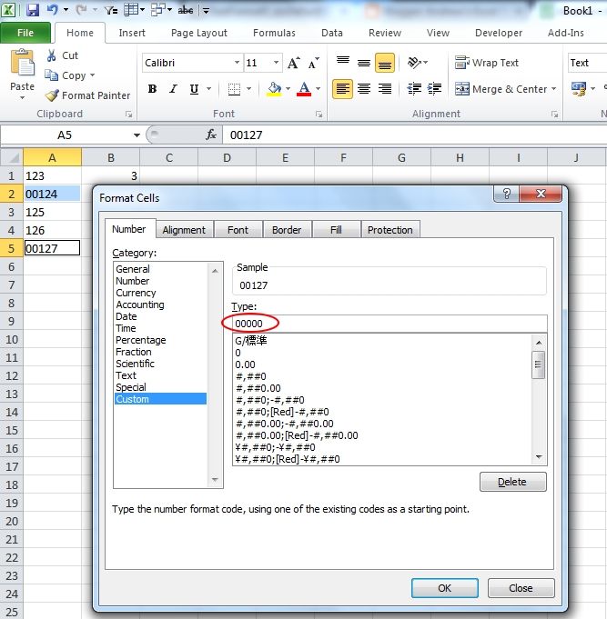
Now it's a matter of choosing a more suitable format. As it turns out, the other cells have been formatted as 00000 to show the numbers as 5 digits. To match this, I select Custom on the Number tab, then type in 00000 and click OK.



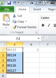
Yay! Hang on... cell B1 still shows a total of 3. Yikes!



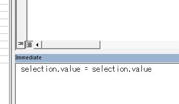
VBA is your friend. Make sure all cells are selected. Type Ctrl + F11 to show the Visual Basic Editor, then Ctrl + G to show the Immediate Window (if not already visible).

Now type

selection.value = selection.value


Click Enter on your keyboard. Now all looks good.



Treat yourself to a well-earned cup of tea or coffee. (The alcohol beverages come after work)

See you next time.

Alternate, Alternate Row Banding

Colouring alternate rows (or row banding) in Excel makes looking at data a lot easier on your eyes. There's so many ways to do it.

Back in the good old days, walking 20 kms to school in a blizzard, we used the below formulas with a suitable conditional format,

For odd rows use,

=ODD(ROW())=ROW()
or

=MOD(ROW(),2)<>0
For even rows use,

=EVEN(ROW())=ROW()
or

=MOD(ROW(),2)=0
Or even better, when using Autofilters,

=MOD(SUBTOTAL(3,A$1:A1),2)=0


(Last week's shopping was rather expensive)

But then along came Tables in 2007, with their automatic row banding making things easier. Gah!

Anyway, different colours for alternate rows is good but wouldn't it be even better if the colours change when values change? And still show different colours for alternate rows?

Here's one way to do it.

You'll need 2 helper columns. Let's say Columns A and B are available and values to decide the colouring starting in cell C1.

In cells A1 and B1, enter 1.

Then in cell A2, enter this,

=IF(C2<>C1,A1+1,A1)


and this in cell B2,

=IF(ISODD(A2),IF(B1=1,2,1),IF(B1=3,4,3))


and drag on down to the bottom of the list.



Now we enter some conditional formatting like this,



And we're finished. Here's a sample workbook.

See you next time.